3.4 Linear Regression - CI, MSE, Split, Cross Validation

#加载必备包
library(ISLR)
library(MASS)
library(tidyverse)

Regression in R

#linearmodel #linearregression #slope #coef

#创建一个线性模型
some_formula <- outcome ~ predictor_1 + predictor_2 
#例子
#medv = housing value, lstat = socio-economic status
lm_ses <- lm(formula = medv ~ lstat, data = Boston)
#查看formula的 intercept and slope
coef(lm_ses)
#解读slope结果
## (Intercept)       lstat 
##  34.5538409  -0.9500494
# for each point increase in lstat, the median housing value drops by 0.95
#得到公式medvi=34.55−0.95∗lstati+ϵi，知道新的lstat可以预测medv
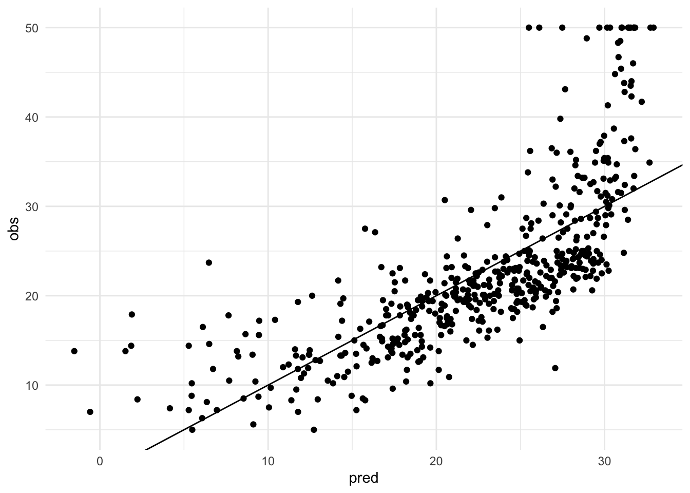
#保存预测的y值
y_pred <- predict(lm_ses)

#观察散点和线性模型的fit程度
tibble(pred = y_pred, 
       obs  = Boston$medv) %>%         #$代表vector
  ggplot(aes(x = pred, y = obs)) +
  geom_point() +
  theme_minimal() +
  geom_abline(slope = 1) #已知理想的线性模型

#生成用于预测的lstat数据
pred_dat <- tibble(lstat = seq(0, 40, length.out = 1000))
#使用新生成的lstat数据放进lm_ses模型预测medv
y_pred_new <- predict(lm_ses, newdata = pred_dat)

Plotting lm() in ggplot

#scatterplot

#把y_pred_new添加到pred_dat dataframe里的medv的方法一
pred_dat$medv <- y_pred_new
#方法二
pred_dat <- pred_dat %>% mutate(medv = y_pred_new) 

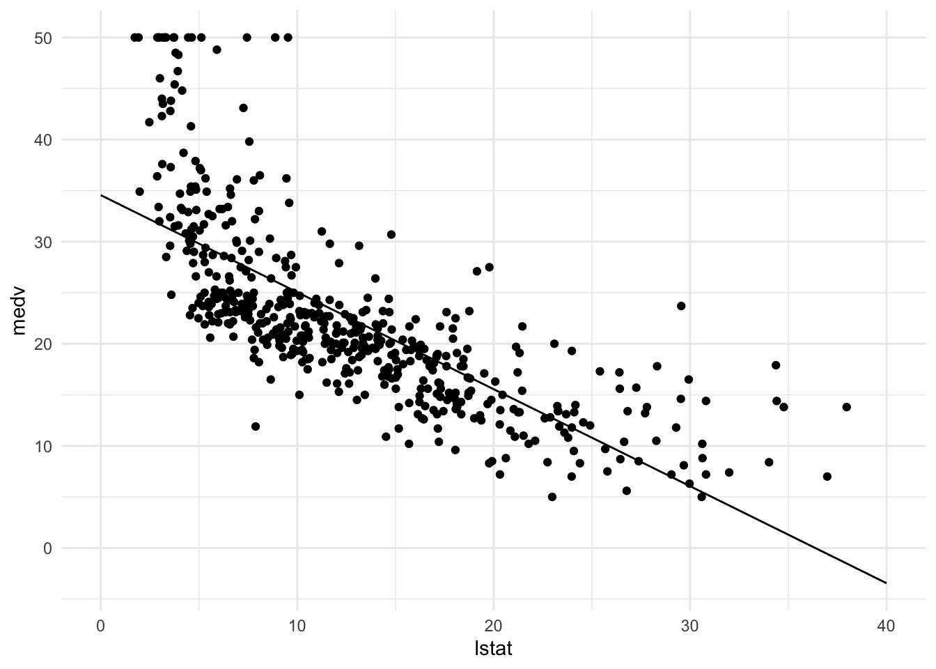
#带有线性模型的散点图（未知理想的线性模型是什么样的，需要计算）
p_scatter <- 
  Boston %>%                             # dataset名称
  ggplot(aes(x = lstat, y = medv)) +
  geom_point() +
  theme_minimal() + 
  p_scatter + geom_line(data = pred_dat)
p_scatter 

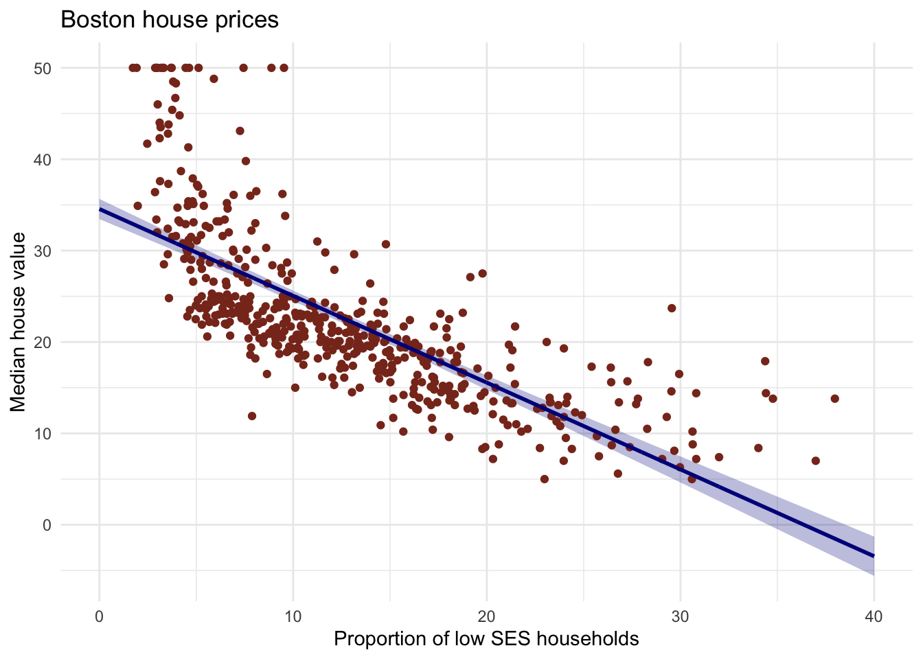
#confidenceintervals #ci

#查看confidence interval
y_pred_95 <- predict(lm_ses, newdata = pred_dat, interval = "confidence")
head(y_pred_95)
# 得到matrix with an estimate and a lower and an upper confidence interval
##        fit      lwr      upr
## 1 34.55384 33.44846 35.65922
## 2 34.51580 33.41307 35.61853
## 3 34.47776 33.37768 35.57784
## 4 34.43972 33.34229 35.53715
## 5 34.40168 33.30690 35.49646
## 6 34.36364 33.27150 35.45578
#根据matrix创建dataframe
gg_pred <- tibble(
  lstat = pred_dat$lstat,
  medv  = y_pred_95[, 1],
  lower = y_pred_95[, 2],
  upper = y_pred_95[, 3]
)
gg_pred

#ribbon #geomribbon

#plot confidence intervals
Boston %>% 
  ggplot(aes(x = lstat, y = medv)) + 
  geom_ribbon(aes(ymin = lower, ymax = upper), data = gg_pred, fill = "#00008b44") +
  geom_point(colour = "#883321") + 
  geom_line(data = pred_dat, colour = "#00008b", size = 1) +
  theme_minimal() + 
  labs(x    = "Proportion of low SES households",
       y    = "Median house value",
       title = "Boston house prices")
#解释：The ribbon represents the 95% confidence interval of the fit line.
# The uncertainty in the estimates of the coefficients are taken into
# account with this ribbon. 

# You can think of it as:
# upon repeated sampling of data from the same population, at least 95% of
# the ribbons will contain the true fit line.

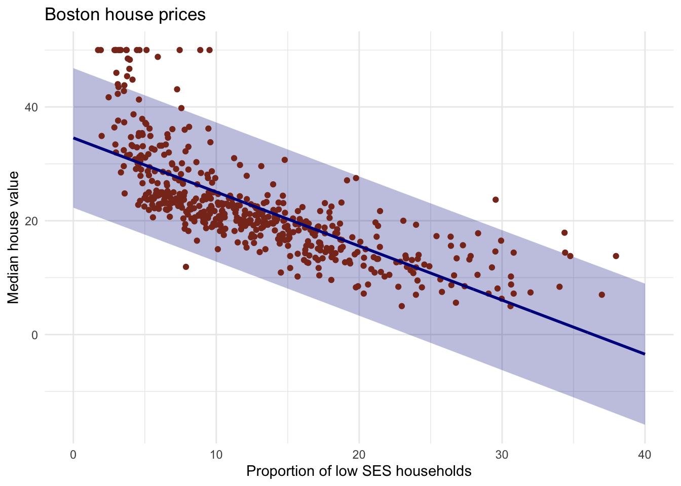
# confidence interval改为pred interval
y_pred_95 <- predict(lm_ses, newdata = pred_dat, interval = "prediction")
# create the df
gg_pred <- tibble(
  lstat = pred_dat$lstat,
  medv  = y_pred_95[, 1],
  l95   = y_pred_95[, 2],
  u95   = y_pred_95[, 3]
)
# Create the plot
Boston %>% 
  ggplot(aes(x = lstat, y = medv)) + 
  geom_ribbon(aes(ymin = l95, ymax = u95), data = gg_pred, fill = "#00008b44") +
  geom_point(colour = "#883321") + 
  geom_line(data = pred_dat, colour = "#00008b", size = 1) +
  theme_minimal() + 
  labs(x     = "Proportion of low SES households",
       y     = "Median house value",
       title = "Boston house prices")

Mean square error

#创建MSE函数
mse <- function(y_true, y_pred) {
  mean((y_true - y_pred)^2)
}
#测试MSE是否正常运行
mse(1:10, 10:1) #结果是33表示正常
#计算lm_ses线性模型的MSE
mse(Boston$medv, predict(lm_ses))

Train-validation-test split

#split #train #validation #test

#把数据添加train, validation, test三个类别vector，总数须等于dataset的observations
splits <- c(rep("train", 253), rep("validation", 152), rep("test", 101))
#随机排列vector数据，把vector添加到Boston dataset里，命名新dataset为boston_master
boston_master <- Boston %>% mutate(splits = sample(splits))
#使用split把一个dataset分成三个
boston_train <- boston_master %>% filter(splits == "train")
boston_valid <- boston_master %>% filter(splits == "validation")
boston_test  <- boston_master %>% filter(splits == "test")

#使用train dataset训练一个线性模型
model_1 <- lm(medv ~ lstat, data = boston_train)
summary(model_1)
#计算该train线性模型的MSE
model_1_mse_train <- mse(y_true = boston_train$medv, y_pred = predict(model_1))
#计算validation dataset线性模型的MSE
model_1_mse_valid <- mse(y_true = boston_valid$medv, 
                         y_pred = predict(model_1, newdata = boston_valid))

#添加age和tax作为predictors（预测用的变量），使用train和valid dataset训练第二个线性模型
model_2 <- lm(medv ~ lstat + age + tax, data = boston_train)
model_2_mse_train <- mse(y_true = boston_train$medv, y_pred = predict(model_2))
model_2_mse_valid <- mse(y_true = boston_valid$medv, 
                         y_pred = predict(model_2, newdata = boston_valid))

#使用test dataset较两个线性模型，看哪个有lower training and validation MSE
model_2_mse_test <- mse(y_true = boston_test$medv, 
                        y_pred = predict(model_2, newdata = boston_test))
sqrt(model_2_mse_test)
#哪个sqrt小说明哪个更accurate

Cross-validation

#crossvalidation

# Create a function that performs k-fold cross-validation for linear models
mse <- function(y_true, y_pred) mean((y_true - y_pred)^2)

cv_lm <- function(formula, dataset, k) {
  # We can do some error checking before starting the function
  stopifnot(is_formula(formula))       # formula must be a formula
  stopifnot(is.data.frame(dataset))    # dataset must be data frame
  stopifnot(is.integer(as.integer(k))) # k must be convertible to int
  
  # first, add a selection column to the dataset as before
  n_samples  <- nrow(dataset)
  select_vec <- rep(1:k, length.out = n_samples)
  data_split <- dataset %>% mutate(folds = sample(select_vec))
  
  # initialise an output vector of k mse values, which we 
  # will fill by using a _for loop_ going over each fold
  mses <- rep(0, k)
  
  # start the for loop
  for (i in 1:k) {
    # split the data in train and validation set
    data_train <- data_split %>% filter(folds != i)
    data_valid <- data_split %>% filter(folds == i)
    
    # calculate the model on this data
    model_i <- lm(formula = formula, data = data_train)
    
    # Extract the y column name from the formula
    y_column_name <- as.character(formula)[2]
    
    # calculate the mean square error and assign it to mses
    mses[i] <- mse(y_true = data_valid[[y_column_name]],
                   y_pred = predict(model_i, newdata = data_valid))
  }
  
  # now we have a vector of k mse values. All we need is to
  # return the mean mse!
  mean(mses)
}

#perform 9-fold cross validation with a linear model with formula medv ~ lstat + age + tax
cv_lm(formula = medv ~ lstat + age + tax, dataset = Boston, k = 9)
[1] 38.14796
cv_lm(formula = medv ~ lstat + I(lstat^2) + age + tax, dataset = Boston, k = 9)
[1] 28.01808
结果说明添加一个higher-order polynomial term like lstat^2可以让模型变得更加精确，因为这样可以capture nonlinear relationships between lstat and medv