3.5 Classification - KNN, Confusion Matrix, LR, LDA (Used For Predicting Categorical Variables)
library(MASS)
library(class)
library(ISLR)
library(tidyverse)
#set seed
set.seed(45)
Default dataset
#scatterplot
#scatterplot
Default %>%
  arrange(default) %>% # so the yellow dots are plotted after the blue ones
  ggplot(aes(x = balance, y = income, colour = default)) +
  geom_point(size = 1.3) +
  theme_minimal() +
  scale_colour_viridis_d() +
  facet_grid(cols = vars(student)) #按照Student这个Boolean value分成两图
#dummyvariable #split
#turn Student variable into dummy variable of 0 and 1
#split data to training and testing
default_df <-
  Default %>%
  mutate(student = ifelse(student == "Yes", 1, 0)) %>%
  mutate(split = sample(rep(c("train", "test"), times = c(8000, 2000))))

default_train <-
  default_df %>%
  filter(split == "train") %>%
  select(-split)

default_test <-
  default_df %>%
  filter(split == "test") %>%
  select(-split)
K-Nearest Neighbours
#prediction #knn
#when k=5, knn预测的数值
knn_5_pred <- knn(
  train = default_train %>% select(-default),
  test  = default_test  %>% select(-default),
  cl    = as_factor(default_train$default),
  k     = 5
)

bind_cols(default_test, pred = knn_5_pred) %>%
  arrange(default) %>%
  ggplot(aes(x = balance, y = income, colour = pred)) +
  geom_point(size = 1.3) +
  scale_colour_viridis_d() +
  theme_minimal() +
  labs(title = "Predicted class (5nn)")

#真实数值
default_test %>%
  arrange(default) %>%
  ggplot(aes(x = balance, y = income, colour = default)) +
  geom_point(size = 1.3) +
  scale_colour_viridis_d() +
  theme_minimal() +
  labs(title = "True class")
#可以看到很多predicted是no的,真实结果却是yes
Confusion matrix
#confusionmatrix #classification #falsepositive
#一种查看classifications是否正确的方法
table(true = default_test$default, predicted = knn_2_pred)
##      predicted
## true    No  Yes
##   No  1899   31假阳性
##   Yes   55   15

#完美的classification应该是这样的
##      predicted
## true    No  Yes
##   No  1930    0
##   Yes    0   70
Logistic regression
#logisticregression
Used to predict the categorical variable (yes/no, true/false, 0/1)
LR is a probabilistic classifier
KNN is a direct classifier: it outputs a probability which can then be used in conjunction with a cutoff (usually 0.5) to classify new observations.
#Use glm() with argument family = binomial to fit a logistic regression model lr_mod to the default_train data.
lr_mod <- glm(default ~ ., family = binomial, data = default_train)
#Visualise the predicted probabilities versus observed class for the training dataset in lr_mod
tibble(observed  = default_train$default,
       predicted = predict(lr_mod, type = "response")) %>%
  ggplot(aes(y = predicted, x = observed, colour = observed)) +
  geom_point(position = position_jitter(width = 0.2), alpha = .3) +
  scale_colour_manual(values = c("dark blue", "orange"), guide = "none") +
  theme_minimal() +
  labs(y = "Predicted probability to default")
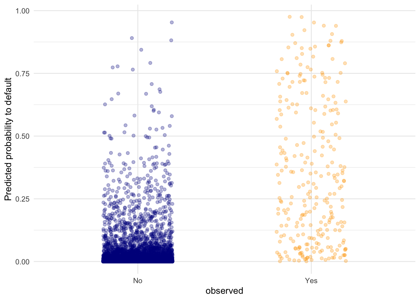
# we can see that the defaulting category has a higher average probability
# for a default compared to the "No" category, but there are still data
# points in the "No" category with high predicted probability for defaulting.
#coefficient
#calculate coefficient for "balance"
coefs <- coef(lr_mod)
coefs["balance"]
#the result is 0.0057.
#The higher the balance, the higher the log-odds of defaulting.
#this means that each dollar increase in balance increases the log-odds by 0.0058

#calculate the probability of default be for a person who is not a student, has an income of 40000, and a balance of 3000 dollars at the end of each month?
logodds <- coefs[1] + 4e4*coefs[4] + 3e3*coefs[3]  #calculate the log-odds
1 / (1 + exp(-logodds))   #convert this to a probability
#the result is 0.998, which means the probability of .998 of defaulting
Visualising the effect of the balance variable
#predict #随机数据
#新建用于预测的随机数据集balance_df with 3 columns and 500 rows: student always 0, balance ranging from 0 to 3000, and income always the mean income in the default_train dataset.
balance_df <- tibble(
  student = rep(0, 500),
  balance = seq(0, 3000, length.out = 500),
  income  = rep(mean(default_train$income), 500)
)

#把新的随机数据集放进之前的LR model,把default概率可视化
balance_df$predprob <- predict(lr_mod, newdata = balance_df, type = "response")
balance_df %>%
  ggplot(aes(x = balance, y = predprob)) +
  geom_line(col = "dark blue", size = 1) +
  theme_minimal()
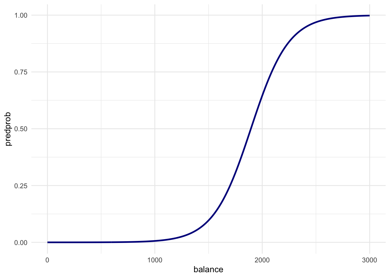
#如何解读该图
# Just before 2000 in the first plot is where the ratio of
# defaults to non-defaults is 50-50. So this line is exactly what we expect!

#绘制LR的confusion matrix
pred_prob <- predict(lr_mod, newdata = default_test, type = "response")
pred_lr   <- factor(pred_prob > .5, labels = c("No", "Yes"))
table(true = default_test$default, predicted = pred_lr)
##      predicted
## true    No  Yes
##   No  1925    5
##   Yes   47   23
Linear discriminant analysis
#LDA
#Train an LDA classifier `lda_mod` on the training set.
lda_mod <- lda(default ~ ., data = default_train)

#how to interpret LDA classifier
lda_mod
## Call:
## lda(default ~ ., data = default_train)
##
## Prior probabilities of groups:
##       No      Yes
## 0.967125 0.032875
##
## Group means:
##       student   balance   income
## No  0.2888717  803.4652 33665.79
## Yes 0.3726236 1749.3143 32559.39
##
## Coefficients of linear discriminants:
##                   LD1
## student -1.452216e-01
## balance  2.231857e-03
## income   5.306987e-06
# defaulters have a larger proportion of students that non-defaulters
# (40% vs 29%), they have a slightly lower income, and they have a
# much higher remaining credit card balance than non-defaulters.

#create confusion matrix to LDA
pred_lda <- predict(lda_mod, newdata = default_test)
table(true = default_test$default, predicted = pred_lda$class)
Predict Titanic survival
#Create a model (using knn, logistic regression, or LDA) to predict whether a 14 year old boy from the 3rd class would have survived the Titanic disaster. You can find the data in the data/ folder. Would the passenger have survived if they were a girl in 2nd class?

titanic <- read_csv("data/Titanic.csv")

lr_mod_titanic <- glm(Survived ~ PClass * Sex * Age, data = titanic)

predict(lr_mod_titanic,
        newdata = tibble(
          PClass = c( "3rd",    "2nd"),
          Age    = c(    14,       14),
          Sex    = c("male", "female")
        ),
        type = "response"
)
##         1         2
## 0.2215689 0.9230483
#拼图
把四个plot拼在一起
library(ggplot2)
library(gridExtra)
grid.arrange(plot1, plot2, plot3, plot4, ncol = 2)