3.6 Classification Evaluation - Confusion Matrix, LR, LDA, Classification Trees, Random Forest

#install.packages() if necessary
library(MASS)
library(ISLR)
library(tidyverse)

library(pROC)

library(rpart)
library(rpart.plot)
library(randomForest)

Confusion matrix, continued

#logisticregression #confusionmatrix #cutoff

#生成confusion matrix
#Create a LR model `lr_mod` for this data using the formula `response ~ .` and create a confusion matrix based on a .5 cutoff probability.

treat <- read_csv("data/cardiovascular_treatment.csv") %>% 
  mutate(severity = as.factor(severity),
         gender   = as.factor(gender),
         dose     = as.factor(dose),
         response = as.factor(response))

lr_mod <- glm(response ~ ., "binomial", treat)


prob_lr <- predict(lr_mod, type = "response")
pred_lr <- ifelse(prob_lr > .5, 1, 0)

table(true = treat$response, pred = pred_lr)

#falsepositive

#计算confusion matrix里的各种概率
cmat_lr <- table(true = treat$response, pred = pred_lr)

TN <- cmat_lr[1, 1]
FN <- cmat_lr[2, 1]
FP <- cmat_lr[1, 2]
TP <- cmat_lr[2, 2]

tibble(
  Acc = (TP + TN) / sum(cmat_lr),
  TPR = TP / (TP + FN),
  TNR = TN / (TN + FP),
  FPR = FP / (TN + FP),
  PPV = TP / (TP + FP),
  NPV = TN / (TN + FN)
)

#解读概率
|Acc<br><br><dbl>|TPR<br><br><dbl>|TNR<br><br><dbl>|FPR<br><br><dbl>|PPV<br><br><dbl>|NPV<br><br><dbl>|
|--:|--:|--:|--:|--:|--:|
|0.6996047|0.7698413|0.6299213|0.3700787|0.6736111|0.733945|

# Accuracy is .7, meaning that 30% of the patients are misclassified

# [TPR] If the patient will respond to treatment, there is an 77% probability 
# that the model will detect this

# [TNR] If the patient will not respond to treatment, there is a 63% prob
# that the model will detect this

# [FPR] If the patient does not respond to treatment, there is a 37% chance
# he or she will anyway be predicted to respond to the treatment

# [PPV] If the patient is predicted to respond to the treatment, there is a
# 67% chance they will actually respond to the treatment

# [NPV] If the patient is predicted to not respond to the treatment, there is
# a 73% probability that they will indeed not respond to the treatment

# The last two metrics are very relevant: if a new patient comes in you will
# only know the prediction and not the true value

#LDA

#使用LDA对同一个dataset进行预测
lda_mod <- lda(response ~ ., treat)
pred_lda <- predict(lda_mod)$class
cmat_lda <- table(true = treat$response, pred = pred_lda)

TN <- cmat_lda[1, 1]
FN <- cmat_lda[2, 1]
FP <- cmat_lda[1, 2]
TP <- cmat_lda[2, 2]

# PPV
PPV <- TP / (TP + FP)
NPV <- TN / (TN + FN)

#LRvsLDA

#比较LR和LDA对新数据集的预测结果
new_patients <- read_csv("data/new_patients.csv") %>% 
  mutate(severity = as.factor(severity),
         gender   = as.factor(gender),
         dose     = as.factor(dose),
         response = as.factor(response))

pred_lda_new <- predict(lda_mod, newdata = new_patients)$class
prob_lr_new <- predict(lr_mod, newdata = new_patients, type = "response")
pred_lr_new <- ifelse(prob_lr_new > .5, 1, 0)

# lda
cmat_lda_new <- table(true = new_patients$response, pred = pred_lda_new)

# lr
cmat_lr_new <- table(true = new_patients$response, pred = pred_lr_new)

cmat_lda_new
##     pred
## true  0  1
##    0 16 11
##    1  9 14

cmat_lr_new
##     pred
## true  0  1
##    0 16 11
##    1  9 14

PPV <- cmat_lda_new[2, 2] / sum(cmat_lda_new[, 2])
NPV <- cmat_lda_new[1, 1] / sum(cmat_lda_new[, 1])
##0.56, 0.64
# Out-of-sample ppv and npv are worse, as expected
# The models perform only slightly above chance level!

#计算out-of-sample brier score for the lr_mod
mean((prob_lr_new - (as.numeric(new_patients$response) - 1)) ^ 2)
## [1] 0.2283307
# the mean squared difference between the probability and the true class is .23

#roc #roccurve

#通过ROC curve比较两个模型的表现
#Create two LR models: lr1_mod with severity, age, and bb_score as predictors, and lr2_mod with the formula response ~ age + I(age^2) + gender + bb_score * prior_cvd * dose. Save the predicted probabilities on the training data.

lr1_mod <- glm(response ~ severity + bb_score + age, 
               family = "binomial", data = treat)
prob_lr1 <- predict(lr1_mod, type = "response")

lr2_mod <- glm(response ~ age + I(age^2) + gender + bb_score * prior_cvd * dose, 
               family = "binomial", data = treat)
prob_lr2 <- predict(lr2_mod, type = "response")

#Use the function roc() from the pROC package to create two ROC objects with the predicted probabilities: roc_lr1 and roc_lr2. Use the ggroc() method on these objects to create an ROC curve plot for each. Which model performs better? Why?

roc_lr1 <- roc(treat$response, prob_lr1)
## Setting levels: control = 0, case = 1
## Setting direction: controls < cases
roc_lr2 <- roc(treat$response, prob_lr2)
## Setting levels: control = 0, case = 1
## Setting direction: controls < cases
ggroc(roc_lr1) + theme_minimal() + labs(title = "LR1")
ggroc(roc_lr2) + theme_minimal() + labs(title = "LR2")

# The LR2 model performs better: at just about every cutoff value, both the
# sensitivity and the specificity are higher than that of the LR1 model.

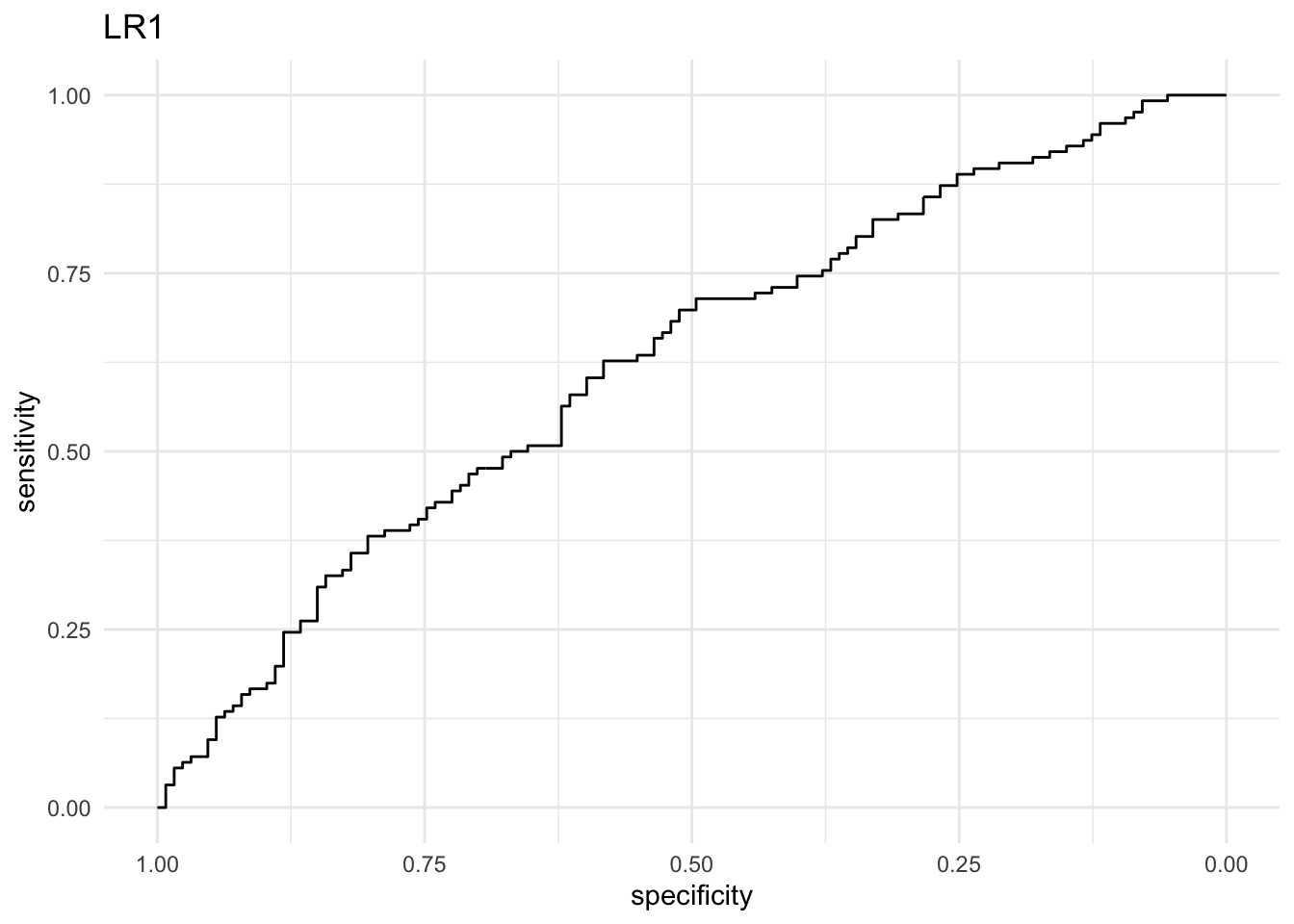
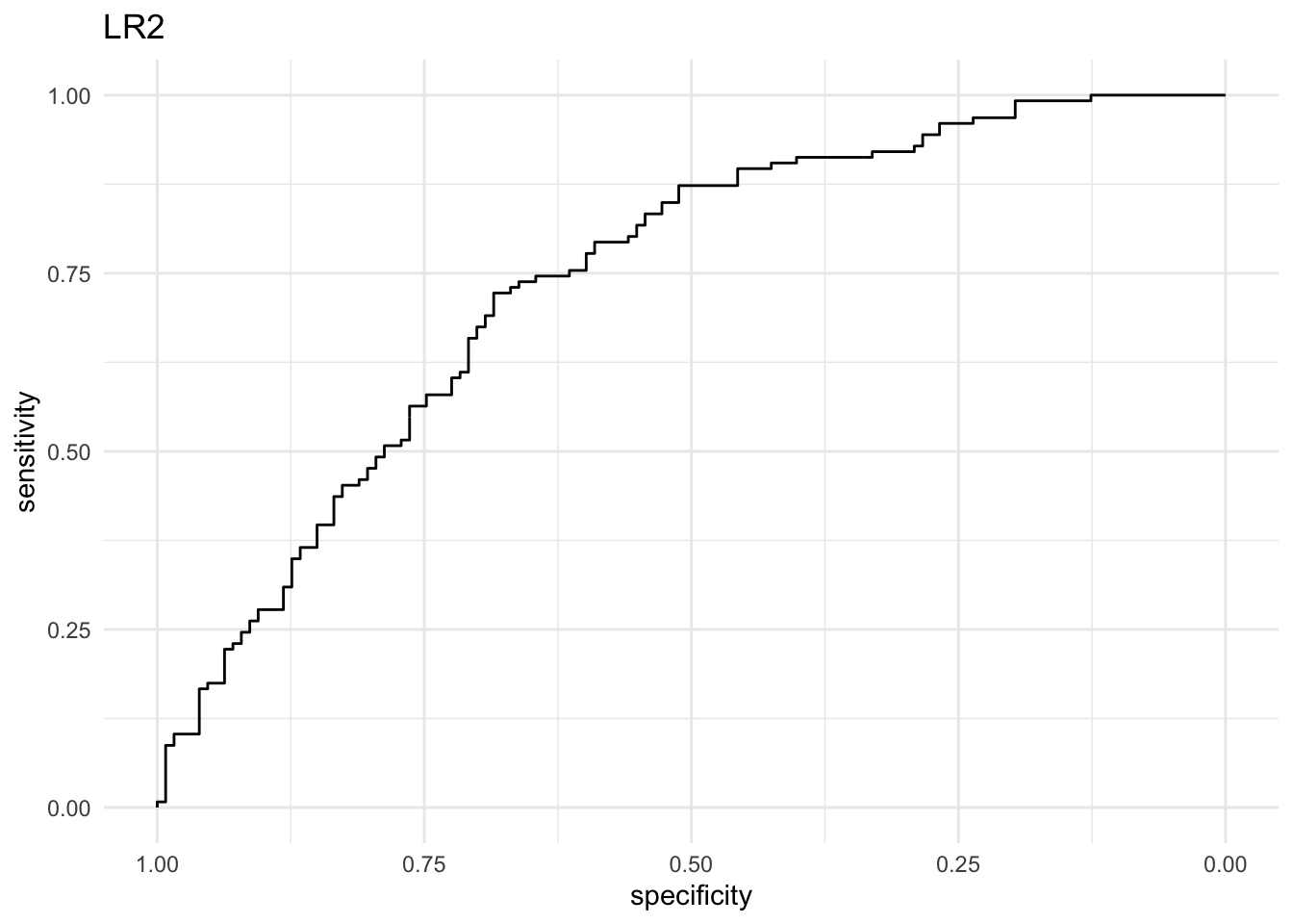
#auc #areaunderthecurve

#比较两个模型的AUC
roc_lr1
roc_lr2
# lr2 has a much higher AUC (area under the ROC curve). It represents the area
# under the curve we drew before. The minimum AUC value is 0.5 and the maximum
# is 1. 

Iris dataset

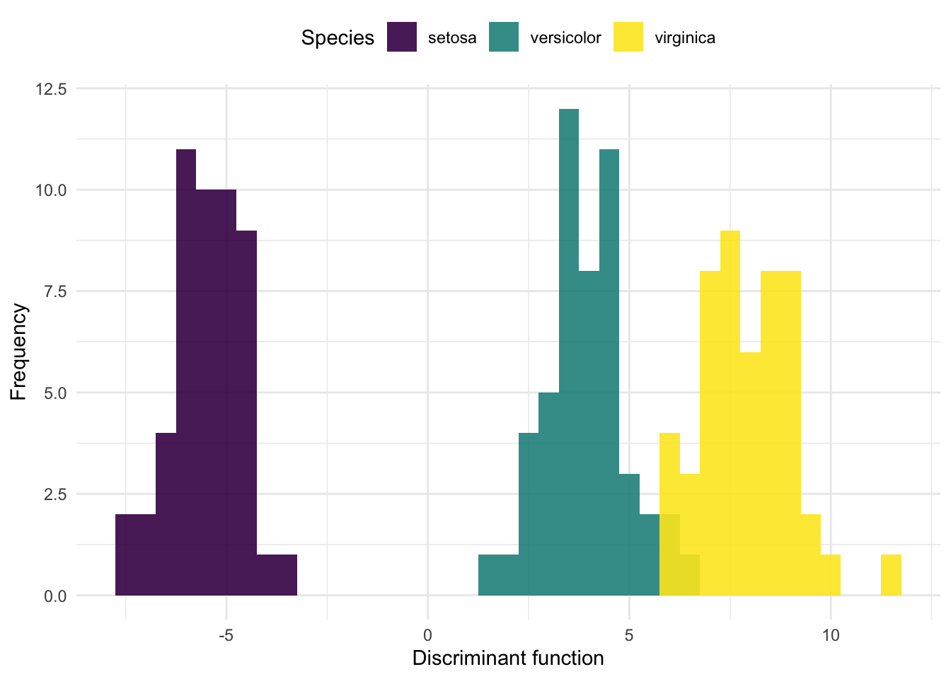
# fit lda model, i.e. calculate model parameters
lda_iris <- lda(Species ~ ., data = iris)

# use those parameters to compute the first linear discriminant
first_ld <- -c(as.matrix(iris[, -5]) %*% lda_iris$scaling[,1])

# plot
tibble(
  ld = first_ld,
  Species = iris$Species
) %>% 
  ggplot(aes(x = ld, fill = Species)) +
  geom_histogram(binwidth = .5, position = "identity", alpha = .9) +
  scale_fill_viridis_d(guide = ) +
  theme_minimal() +
  labs(
    x = "Discriminant function",
    y = "Frequency", 
    main = "Fisher's linear discriminant function on Iris species"
  ) + 
  theme(legend.position = "top")

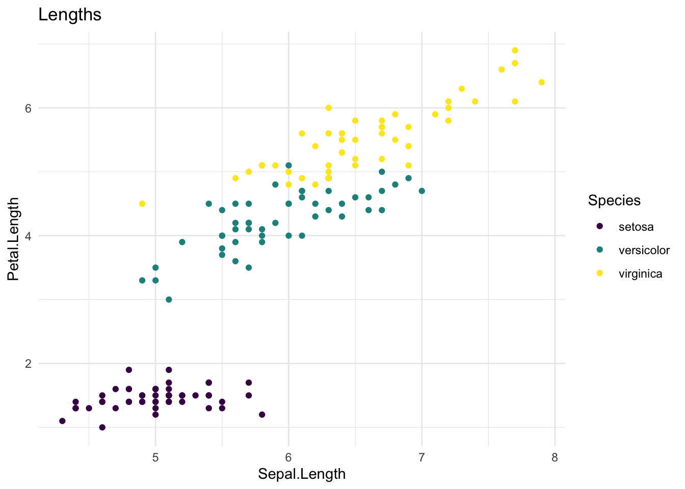
# Some example plots you could make
iris %>% 
  ggplot(aes(x = Sepal.Length, y = Petal.Length, colour = Species)) + 
  geom_point() +
  scale_colour_viridis_d() +
  theme_minimal() +
  ggtitle("Lengths")

#Fit an additional LDA model, but this time with only Sepal.Length and Sepal.Width as predictors.
lda_iris_sepal <- lda(Species ~ Sepal.Length + Sepal.Width, data = iris)

#Create a confusion matrix of the lda_iris and lda_iris_sepal models. (NB: we did not split the dataset into training and test set, so use the training dataset to generate the predictions.). Which performs better in terms of accuracy?
# lda_iris
table(true = iris$Species, predicted = predict(lda_iris)$class)
##             predicted
## true         setosa versicolor virginica
##   setosa         50          0         0
##   versicolor      0         48         2
##   virginica       0          1        49
# lda_iris_sepal
table(true = iris$Species, predicted = predict(lda_iris_sepal)$class)
##             predicted
## true         setosa versicolor virginica
##   setosa         49          1         0
##   versicolor      0         36        14
##   virginica       0         15        35
# lda_iris performs better: sum(off-diagonal) is lower.

#拼图
install.packages("gridExtra")
library(gridExtra)
grid.arrange(LR1, LR2, ncol = 2)

Classification trees

#classification #classificationtrees #分类树

#新建classification trees
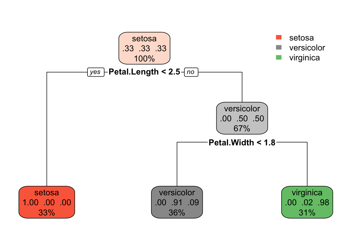
#Use rpart() to create a classification tree for the Species of iris. Call this model iris_tree_mod. Plot this model using rpart.plot().
iris_tree_mod <- rpart(Species ~ ., data = iris)
rpart.plot(iris_tree_mod)

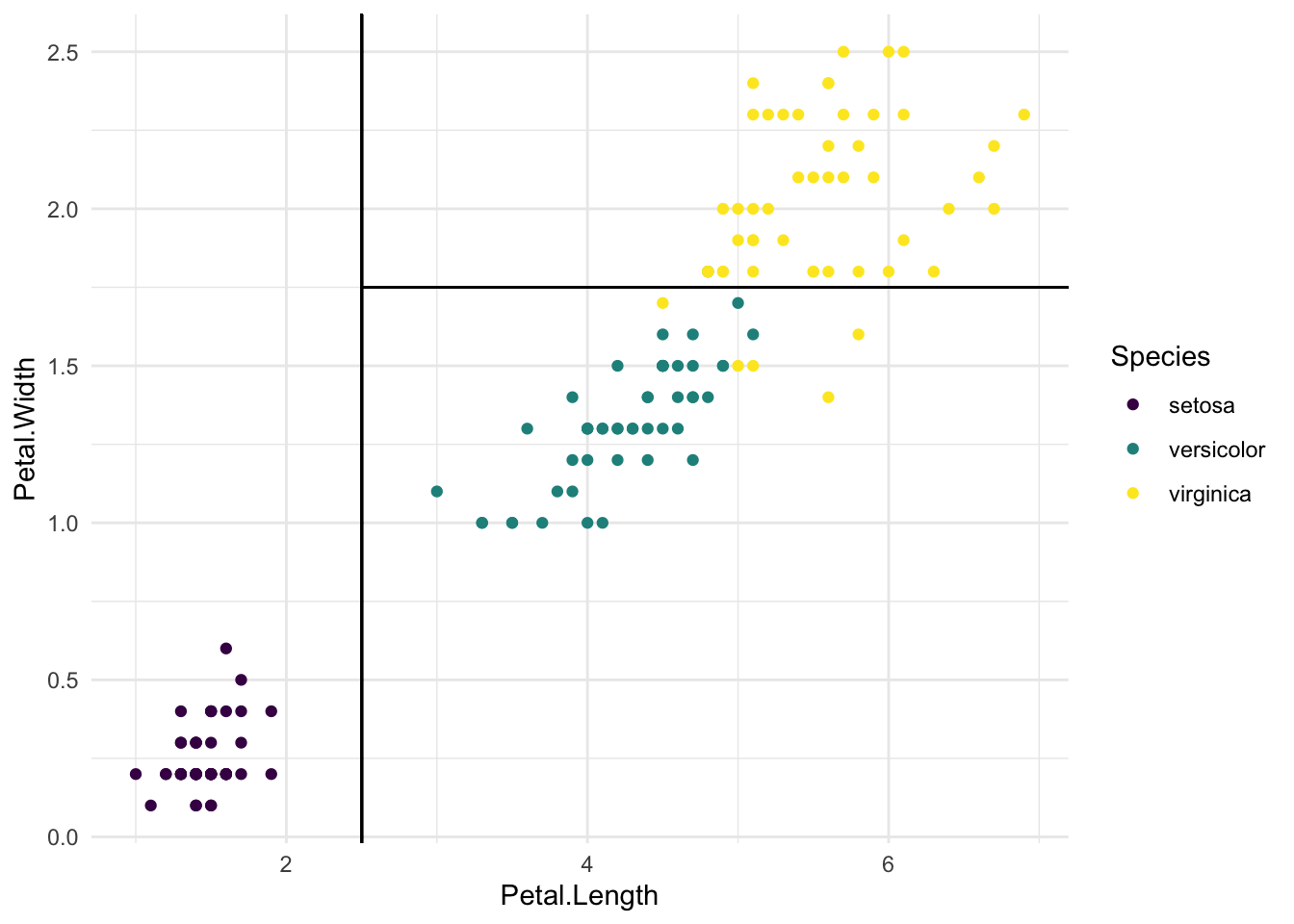
#散点图新建竖线表示分类树
iris %>% 
  ggplot(aes(x = Petal.Length, y = Petal.Width, colour = Species)) +
  geom_point() +
  geom_segment(aes(x = 2.5, xend = 2.5, y = -Inf, yend = Inf),
               colour = "black") +
  geom_segment(aes(x = 2.5, xend = Inf, y = 1.75, yend = 1.75), 
               colour = "black") +
  scale_colour_viridis_d() +
  theme_minimal()

#读图
# The first split perfectly separates setosa from the other two
# the second split leads to 5 misclassifications: 
# virginica classified as versicolor

#新建最详细的分类树
iris_tree_full_mod <- rpart(Species ~ ., data = iris, 
                            control = rpart.control(minbucket = 1, cp = 0))

rpart.plot(iris_tree_full_mod)

Random forest for classification

#randomforest #随机森林

#使用随机森林检测各个变量的重要性
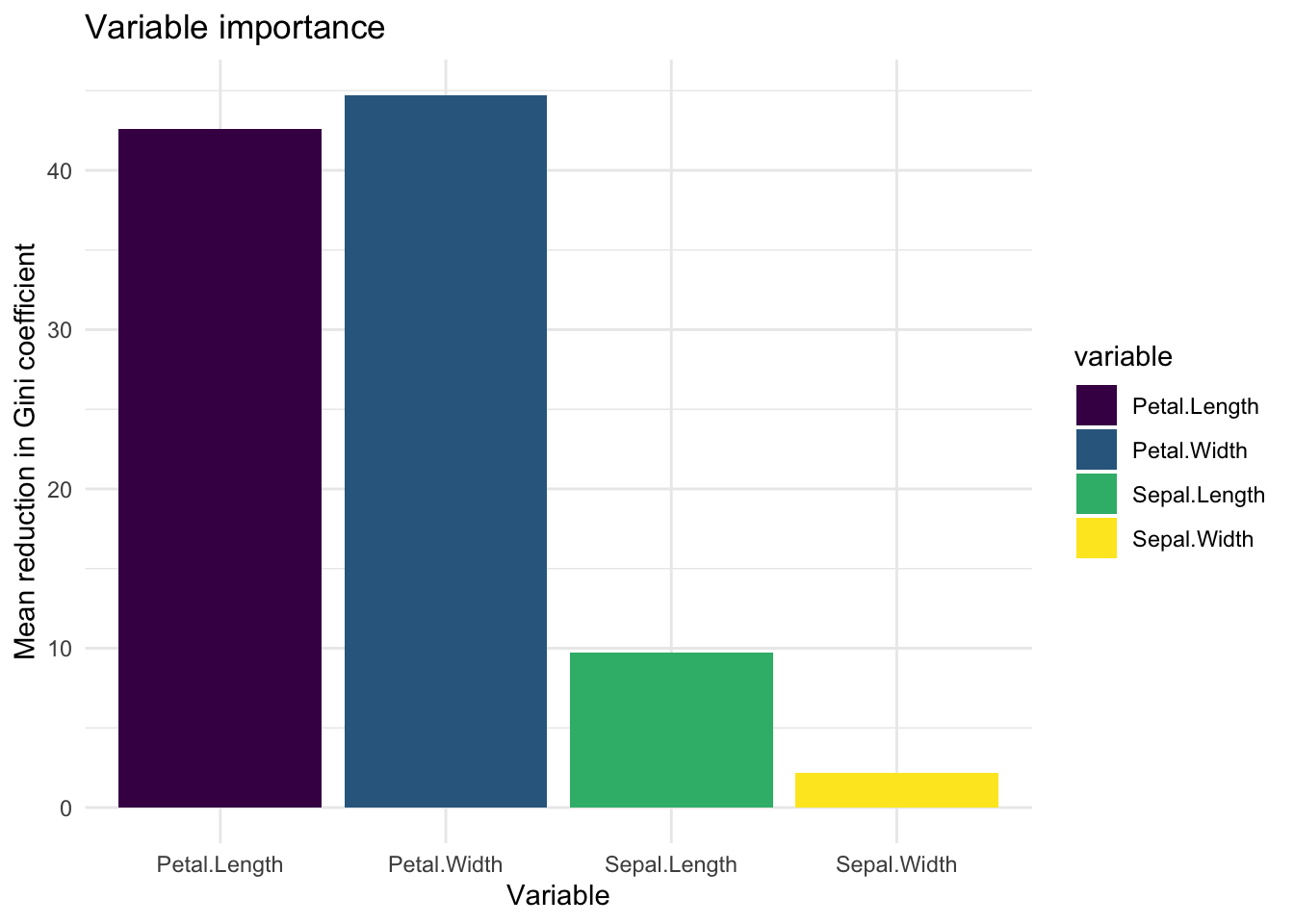
#Use the function randomForest() to create a random forest model on the iris dataset. Use the function importance() on this model and create a bar plot of variable importance. Does this agree with your expectations? How well does the random forest model perform compared to the lda_iris model?

rf_mod <- randomForest(Species ~ ., data = iris)

var_imp <- importance(rf_mod)
tibble(
  importance = c(var_imp), 
  variable = rownames(var_imp)
) %>% 
  ggplot(aes(x = variable, y = importance, fill = variable)) +
  geom_bar(stat = "identity") +
  scale_fill_viridis_d() +
  theme_minimal() +
  labs(
    x = "Variable", 
    y = "Mean reduction in Gini coefficient", 
    title = "Variable importance"
  )