3.7 Nonlinear Regression - Prediction Plot, Poly

install.packages("splines")

library(MASS)
library(splines)
library(ISLR)
library(tidyverse)

set.seed(45)

Prediction plot

#predictionplot

#Create a function called pred_plot() that takes as input an lm object
pred_plot <- function(model) {
  # First create predictions for all values of lstat
  x_pred <- seq(min(Boston$lstat), max(Boston$lstat), length.out = 500)
  y_pred <- predict(model, newdata = tibble(lstat = x_pred))
  
  # Create a ggplot object with a line based on those predictions
  Boston %>%
    ggplot(aes(x = lstat, y = medv)) +
    geom_point() +
    geom_line(data = tibble(lstat = x_pred, medv = y_pred), size = 1, col = "blue") +
    theme_minimal()
}

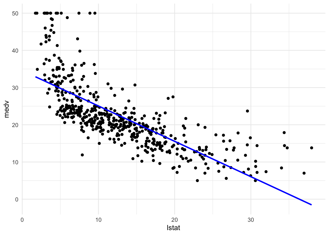
#Create a linear regression object called lin_mod which models medv as a function of lstat
lin_mod <- lm(medv ~ lstat, data = Boston)
pred_plot(lin_mod)

Polynomial regression

#polynomial #polynomialregression

pn3_mod <- lm(medv ~ lstat + I(lstat^2) + I(lstat^3), data = Boston)
pred_plot(pn3_mod)
#适合想要有更多控制的情况，因为可以只选一次方和三次方，而不选二次方

pn3_mod2 <- lm(medv ~ poly(lstat, 3, raw = TRUE), data = Boston)
pred_plot(pn3_mod2)
#poly()适合想要更简洁的情况，因为不能自主设定选几个不同的次方

Piecewise regression

#piecewise #piecewiseregression
适合情况：relationship between variables might change abruptly at a certain threshold，比如农作物低于某个气温，产量有很大变化
#设定用于分成几个piece的数值

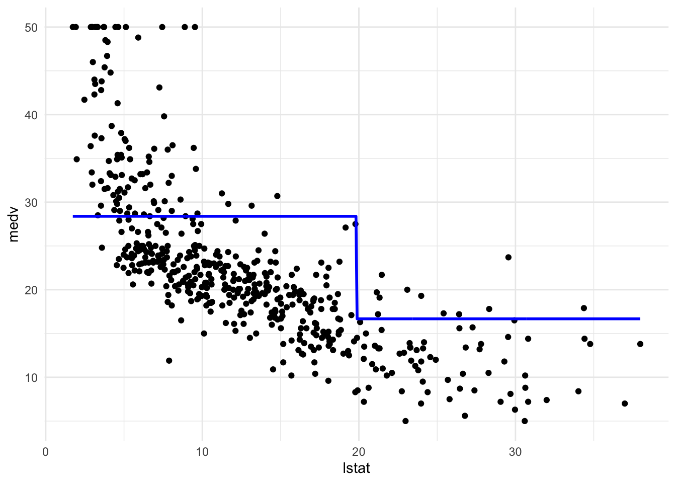
#Create a model called pw2_mod with one predictor: I(lstat <= median(lstat)). 
#Create a pred_plot with this model. 
#Use the coefficients in coef(pw2_mod) to find out what the predicted value for a low-lstat neighbourhood is.

pw2_mod <- lm(medv ~ I(lstat <= median(lstat)), data = Boston)
pred_plot(pw2_mod)

coef(pw2_mod)
##                   (Intercept) I(lstat <= median(lstat))TRUE 
##                      16.67747                      11.71067
# the predicted value for low-lstat neighbourhoods is 16.68 + 11.71 = 28.39

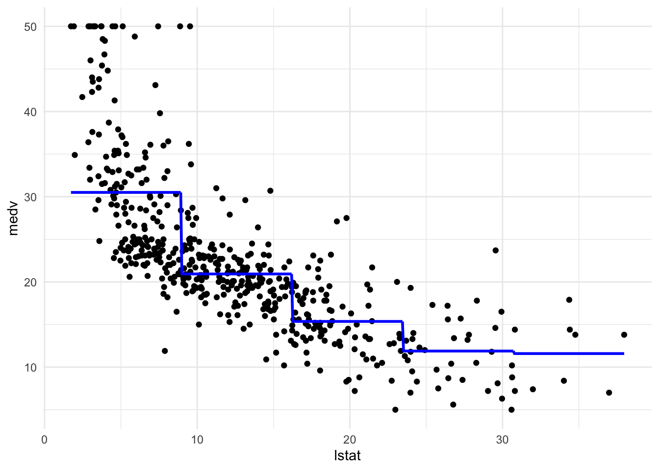
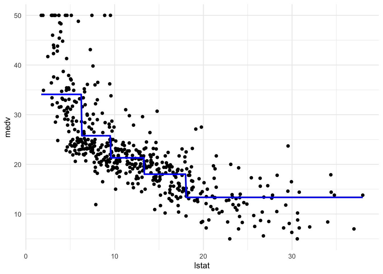
#设定分成n个（space相同的）piece

pw5_mod <- lm(medv ~ cut(lstat, 5), data = Boston)
pred_plot(pw5_mod)

#设定分成n个（datapoint相同的）piece

brks <- c(-Inf, quantile(Boston$lstat, probs = c(.2, .4, .6, .8)), Inf)
pwq_mod <- lm(medv ~ cut(lstat, brks), data = Boston)
pred_plot(pwq_mod)

Piecewise polynomial regression

见https://dgoretzko.github.io/slv/practicals/08_nonlinear_regression/08_nonlinear_regression_answers.html

Splines

#dataframe #splines #ifelse

#create data frame from dataset
boston_tpb <- Boston %>% as_tibble %>% select(medv, lstat)

#added squared lstat and cubed lstat
boston_tpb <- boston_tpb %>% mutate(lstat2 = lstat^2, lstat3 = lstat^3)

#add a column lstat_tpb which is 0 below the median and has value (lstat - median(lstat))^3 above the median.
#ifelse的语法：(condition, true_value, false_value)
boston_tpb <- boston_tpb %>% 
  mutate(lstat_tpb = ifelse(lstat >  median(lstat), (lstat - median(lstat))^3, 0))

#cubicsplinemodel #naturalcubicsplinemodel

#Create a linear model tpb_mod using the lm() function
tpb_mod <- lm(medv ~ lstat + lstat2 + lstat3 + lstat_tpb, data = boston_tpb)
summary(tpb_mod)

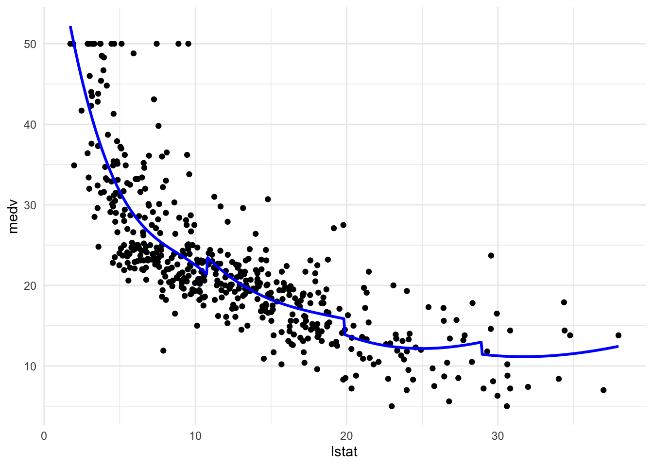
#Create a cubic spline model bs1_mod with a knot at the median using the bs() function.
bs1_mod <- lm(medv ~ bs(lstat, knots = median(lstat)), data = Boston)
summary(bs1_mod)

#plot
#Create a prediction plot from the bs1_mod object using the plot_pred() function.
pred_plot(bs1_mod)

#Create a natural cubic spline model (ns3_mod) with 3 degrees of freedom using the ns() function. 
ns3_mod <- lm(medv ~ ns(lstat, df = 3), data = Boston)
pred_plot(ns3_mod)

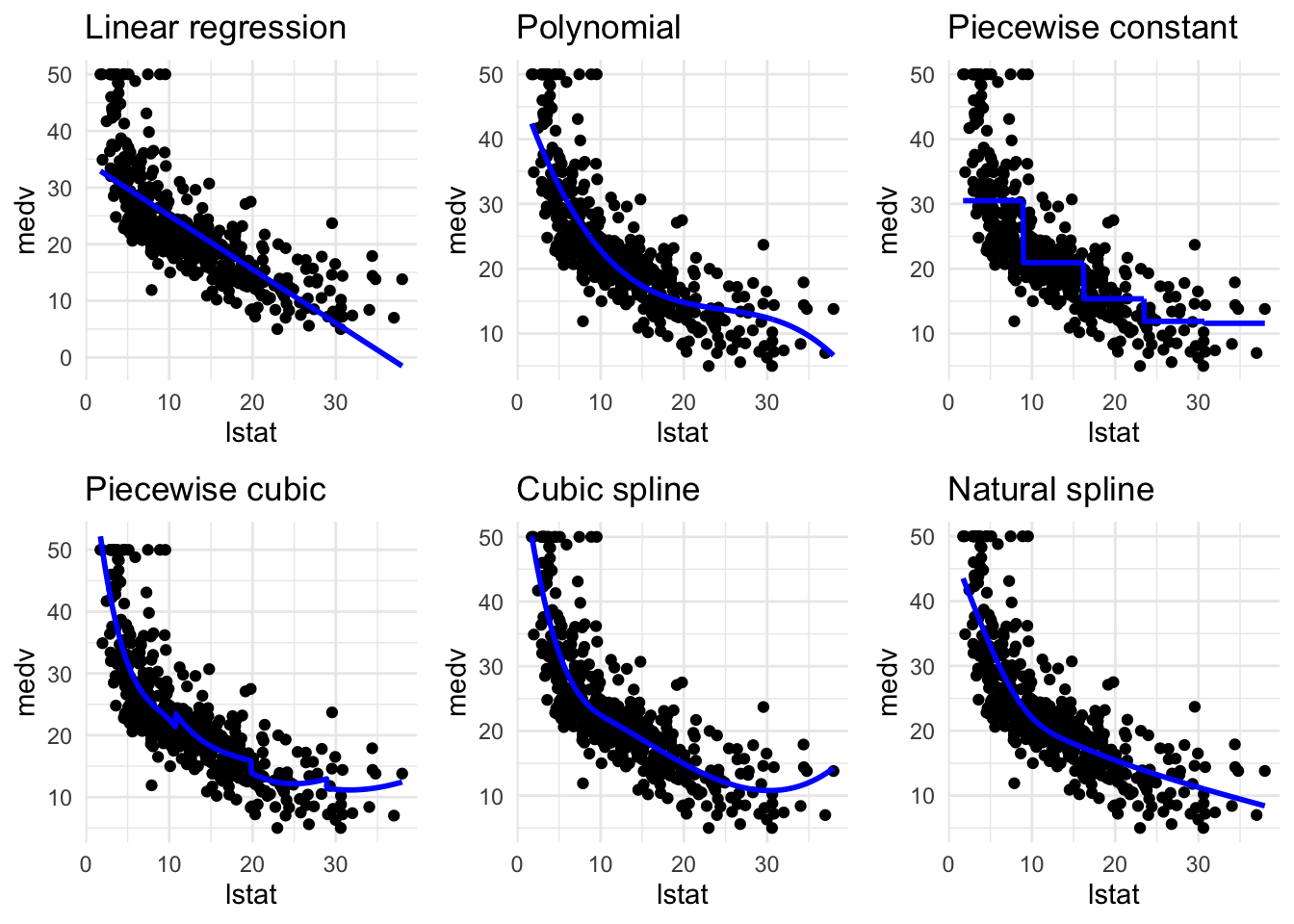
#比较多个plot
library(cowplot)
plot_grid(
  pred_plot(lin_mod) + ggtitle("Linear regression"),
  pred_plot(pn3_mod) + ggtitle("Polynomial"),
  pred_plot(pw5_mod) + ggtitle("Piecewise constant"),
  pred_plot(pc3_mod) + ggtitle("Piecewise cubic"),
  pred_plot(bs1_mod) + ggtitle("Cubic spline"),
  pred_plot(ns3_mod) + ggtitle("Natural spline")
)

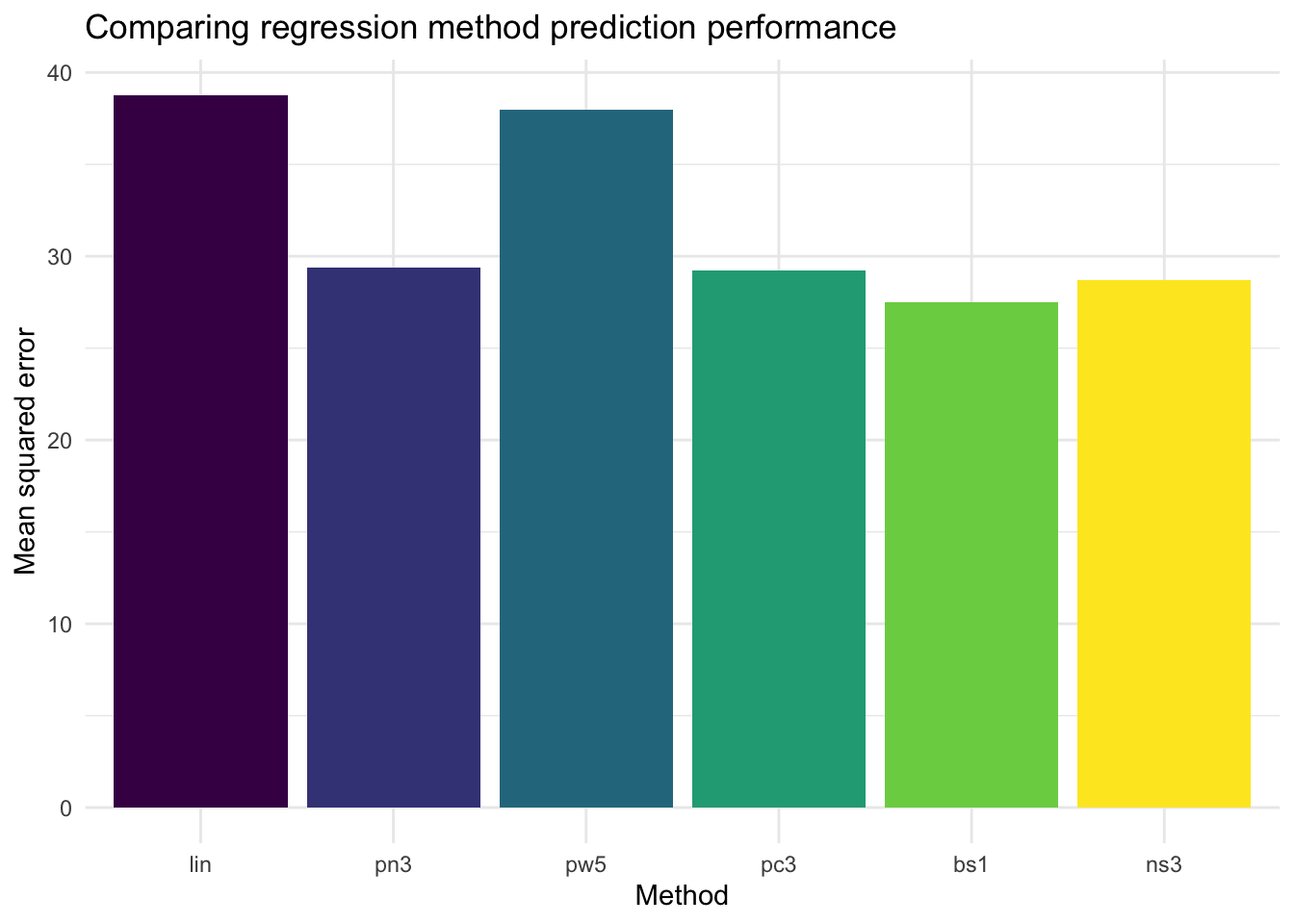
通过计算MSE评价各个模型的表现：

mse <- function(y_true, y_pred) mean((y_true - y_pred)^2)

# add a 12 split column to the boston dataset so we can cross-validate
boston_cv <- Boston %>% mutate(split = sample(rep(1:12, length.out = nrow(Boston))))

# prepare an output matrix with 12 slots per method for mse values
output_matrix <- matrix(nrow = 12, ncol = 6) 
colnames(output_matrix) <- c("lin", "pn3", "pw5", "pc3", "bs1", "ns3")

# loop over the splits, run each method, and return the mse values
for (i in 1:12) {
  train <- boston_cv %>% filter(split != i)
  test  <- boston_cv %>% filter(split == i)
  
  brks <- c(-Inf, 7, 15, 22, Inf)
  
  lin_mod <- lm(medv ~ lstat,                            data = train)
  pn3_mod <- lm(medv ~ poly(lstat, 3),                   data = train)
  pw5_mod <- lm(medv ~ cut(lstat, brks),                 data = train)
  pc3_mod <- lm(medv ~ piecewise_cubic_basis(lstat, 3),  data = train)
  bs1_mod <- lm(medv ~ bs(lstat, knots = median(lstat)), data = train)
  ns3_mod <- lm(medv ~ ns(lstat, df = 3),                data = train)
  
  output_matrix[i, ] <- c(
    mse(test$medv, predict(lin_mod, newdata = test)),
    mse(test$medv, predict(pn3_mod, newdata = test)),
    mse(test$medv, predict(pw5_mod, newdata = test)),
    mse(test$medv, predict(pc3_mod, newdata = test)),
    mse(test$medv, predict(bs1_mod, newdata = test)),
    mse(test$medv, predict(ns3_mod, newdata = test))
  )
}

# this is the comparison of the methods
colMeans(output_matrix)

##      lin      pn3      pw5      pc3      bs1      ns3 
## 38.76726 29.36707 37.95038 29.22791 27.51021 28.68858

# we can show it graphically too
tibble(names = as_factor(colnames(output_matrix)), 
       mse   = colMeans(output_matrix)) %>% 
  ggplot(aes(x = names, y = mse, fill = names)) +
  geom_bar(stat = "identity") +
  theme_minimal() +
  scale_fill_viridis_d(guide = "none") +
  labs(
    x     = "Method", 
    y     = "Mean squared error", 
    title = "Comparing regression method prediction performance"
  )